Cheat Sheet: Build a Comprehensive RAG Application

FAISS vs Chroma DB Comparison

FAISS (Facebook AI Similarity Search)

FAISS is a library developed by Meta for fast vector search that runs on a single machine using either CPU or GPU.

Key Characteristics:

• Type: Library for vector search operations

• Deployment: Single-node operation, no native distributed scaling

• Usage: Code-based integration, no server component

• Control: Full control over indexing and performance

• Metadata: No native metadata support

• Integration: Works with LangChain and LlamaIndex

Chroma DB

Chroma DB is a vector database built for AI use cases that stores both vectors and metadata like tags or descriptions. It can be run locally or as a server.

Key Characteristics:

• Type: Full vector database

• Deployment: Supports both single-node and distributed deployments

• Scaling: Clear path to scale for larger workloads

• Metadata: Native support for storing and filtering metadata

• Indexing: Only supports HNSW (Hierarchical Navigable Small World)

• Integration: Works well with tools like LangChain, easy to integrate

Technology Comparison Summary

• FAISS: Library vs. Chroma DB: Full database

• FAISS: Single-node only vs. Chroma DB: Single-node and distributed

• FAISS: Many indexing options vs. Chroma DB: HNSW only

• FAISS: No native metadata support vs. Chroma DB: Metadata support and filtering

• Both: Work with LangChain and LlamaIndex

FAISS Index Types

Flat Index

A flat index compares the distance (using either Euclidean distance or dot product) between the query embedding and every vector in the vector store using brute force search.

Characteristics:

• Method: Brute force comparison with all vectors

• Accuracy: Very accurate approach

• Performance: Very slow for large datasets

• Use Case: Small datasets where accuracy is critical

Inverted File Index (IVF)

An IVF index speeds up vector search by clustering vectors using methods like k-means, forming Voronoi cells around centroids. Each cell contains vectors closest to its centroid.

Technical Process:

• Clustering: Vectors grouped using k-means into Voronoi cells

• Search Strategy: Query searches only nearest cells, reducing computations

• Trade-off: Faster than flat index but may slightly reduce accuracy

• Limitation: Some nearby vectors might be in other cells

Locality-Sensitive Hashing (LSH)

LSH uses hash functions to map similar vectors to the same bucket, allowing for fast and memory-efficient search.

Characteristics:

• Method: Hash functions group similar vectors into buckets

• Performance: Fast and memory-efficient

• Best Use: High-dimensional sparse data such as text embeddings

• Trade-off: Neither the fastest nor the most accurate method

• Search Process: Searches vectors in closest matching groups

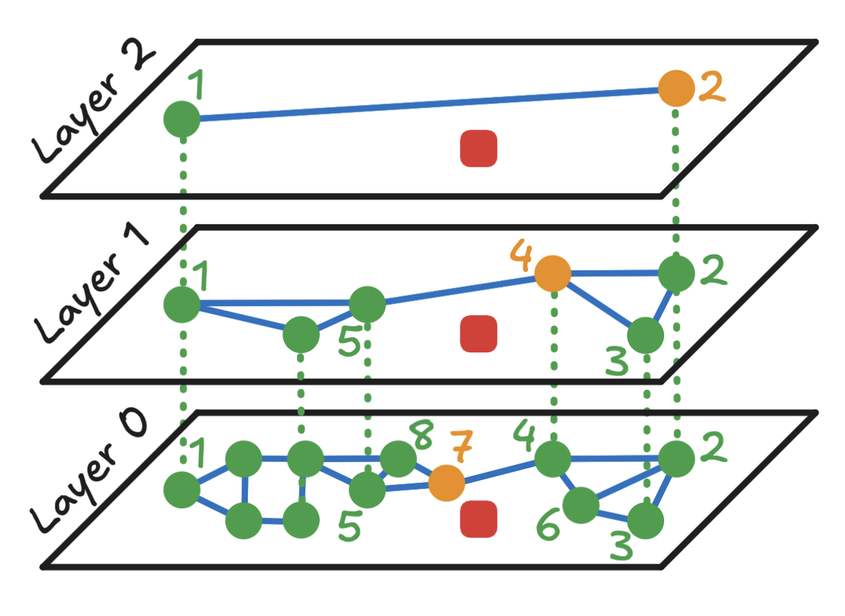
Hierarchical Navigable Small World (HNSW)

HNSW organizes vectors into a hierarchy of layers where top layers are sparse with few vectors acting like express highways, helping the search algorithm quickly approach the target region.

Architecture:

• Top Layers: Sparse, contain only a few vectors (express highways)

• Lower Layers: Denser graphs with detailed local connections

• Search Process: Begins at topmost layer, moves downward using best candidate from each layer

• Performance: Both fast and accurate, especially for large datasets

HNSW Deep Dive

How HNSW Works - Technical Process

The algorithm constructs a multi-layer graph where each layer contains progressively more data points with shorter-range connections:

1. Top Layer Entry: Search begins at the highest layer with sparse, long-range connections

2. Greedy Search: At each layer, move to the neighbor closest to the target query

3. Layer Descent: When no closer neighbors exist, descend to the next layer

4. Progressive Refinement: Graph becomes denser as search descends to lower layers

5. Bottom Layer: Layer 0 contains all data points for final precise search

6. Result: Returns approximate nearest neighbors with high accuracy

Navigation Analogy: Like finding a restaurant in a city - start with highways for long jumps, then use local streets for precise location. The algorithm "zooms in" progressively from major connections to fine-grained local connections.

Key Parameters

M (Max Connections)

• Purpose: Controls how many neighbors each point connects to

• Trade-off: Higher M = better accuracy, more memory usage

• Impact: Lower M = faster build, less memory, lower accuracy

efConstruction (Search Breadth During Build)

• Purpose: Controls how many candidates are considered when finding neighbors during insertion

• Trade-off: Higher efConstruction = better graph quality, slower build

• Impact: Lower efConstruction = faster build, but possibly lower search quality later

efSearch (Search Breadth During Querying)

• Purpose: Controls how many candidate nodes are explored during a query

• Trade-off: Higher efSearch = better accuracy, slower search

• Impact: Main method to tune speed vs. accuracy at query time

ml (Level Multiplier)

• Purpose: Affects how likely a point is to appear in higher layers

• Impact: Controls the shape of the hierarchy

HNSW Limitations

Approximate Results

• Accuracy: HNSW delivers fast results with typical recall rates of 90% to 99%

• Trade-off: May occasionally miss the exact nearest neighbor

• Benefit: For most applications, this trade-off is worthwhile

HNSW and Dynamic Updates

• HNSW is best suited for: Mostly-static datasets

• Challenges: Frequent insertions and deletions can degrade the HNSW index's performance over time

• Solution: Periodic reconstruction may be needed for optimal performance

Distance Metric Limitations

• Works best with: Euclidean distance (L2) and Cosine similarity

• Other metrics: May require modifications or perform suboptimally

Extending FAISS with Milvus

FAISS Limitations

FAISS is effective for local, high-performance vector search, but it lacks features like metadata support and distributed scaling.

Milvus Integration

Milvus, a vector database, uses FAISS as one of its core indexing engines while adding missing capabilities:

• Metadata Support: Storing and filtering metadata alongside vectors

• Hybrid Queries: Enables queries such as "Find similar items under $50"

• Distributed Deployments: Suitable for large-scale production environments

• Scalability: Addresses FAISS's single-node limitation

When to Use Each Technology

Use FAISS When:

• You want full control and performance on a single machine

• You need access to multiple indexing algorithms

• You're building custom, high-performance applications

• Metadata support is not required or can be handled externally

Use Chroma DB When:

• You need quick AI development and prototyping

• Metadata-rich queries are important

• You want easy integration with AI tools

• You need both single-node and distributed deployment options

Use Milvus When:

• You need a scalable, production-ready vector database

• Hybrid search capabilities are desired

• Distributed capabilities are essential

• You want FAISS-level performance with database features

Key Concepts Summary

Index Selection Strategy

Each FAISS index type balances speed, memory, and accuracy differently:

• Flat: Most accurate, slowest (suitable only for small datasets)

• IVF: Balanced speed/accuracy (effective for medium to large datasets, but may be outperformed by HNSW in many cases)

• LSH: Memory-efficient (best for high-dimensional sparse data, though less commonly used)

• HNSW: Fast and accurate (preferred for medium to large datasets due to strong performance and scalability)

HNSW Algorithm Benefits

• Hierarchical Structure: Multi-layer approach enables O(log n) search complexity

• Performance: 90-99% recall rates with fast search times

• Scalability: Especially effective for large datasets

• Flexibility: Tunable parameters for different speed/accuracy requirements

Technology Integration

• Both FAISS and Chroma DB: Work with LangChain and LlamaIndex for RAG pipelines

• Make a choice based on: Project size, complexity, and infrastructure requirements

• Extension options: Milvus uses FAISS under the hood, but provides additional capabilities