Sequence Models
Developer | Adept in software development | Building expertise in machine learning and deep learning
Learning Objectives
Define notation for building sequence models
Describe the architecture of a basic RNN
Identify the main components of an LSTM
Implement backpropagation through time for a basic RNN and an LSTM
Give examples of several types of RNN
Build a character-level text generation model using an RNN
Store text data for processing using an RNN
Sample novel sequences in an RNN
Explain the vanishing/exploding gradient problem in RNNs
Apply gradient clipping as a solution for exploding gradients
Describe the architecture of a GRU
Use a bidirectional RNN to take information from two points of a sequence
Stack multiple RNNs on top of each other to create a deep RNN
Use the flexible Functional API to create complex models
Generate your own jazz music with deep learning
Apply an LSTM to a music generation task
A type of machine learning model designed to handle data that comes in sequences.
Notation
define notation that we will use to build up these sequence model.
x: standing for the input element for the current current time step.
y: standing for the model output for the current current time step.
Tx : denoting the size of time step for input sequence.
Ty : denoting the size of time step for output sequence.
Superscript [𝑙] denotes an object associated with the 𝑙𝑡ℎ layer.
Superscript (𝑖) denotes an object associated with the 𝑖𝑡ℎ example(training set).
Superscript ⟨𝑡⟩ denotes an object at the 𝑡𝑡ℎ time step(time step index).
Subscript 𝑖 denotes the 𝑖𝑡ℎ entry of a vector.
Named-Entity Recognition (NER), which is a key part of sequence models in Natural Language Processing (NLP).
Named-Entity Recognition is like teaching a computer to recognize names in a sentence, just like how we identify people, places, or organizations in our daily conversations. For example, if we take the sentence "Harry Potter and Hermione Granger invented a new spell," NER helps the computer understand that "Harry Potter" and "Hermione Granger" are names of characters. This is important for search engines and other applications that need to organize and index information about people, companies, and locations.
Representing words by one hot vector;
Imagine a giant scoreboard where each word has its own position. If the word is "Harry," we put a "1" in Harry's position and "0s" everywhere else. This way, the computer can easily identify and process each word in the sentence.
Recurrent Neural Network Model
The term "Recurrent" in Recurrent Neural Networks (RNNs) refers to the way the network processes sequences of data by using feedback connections. Here are the key reasons for this naming:
Feedback Loop:
- RNNs have connections that allow information to be fed back into the network. Specifically, the hidden state from the previous time step is used as input for the current time step. This feedback loop enables the network to maintain a memory of previous inputs.
Sequential Processing:
- RNNs process data in a sequential manner, where each time step's output depends not only on the current input but also on the previous hidden state. This recurrent structure allows the network to learn patterns and dependencies over time.
Temporal Dynamics:
- The recurrent nature of RNNs makes them well-suited for tasks involving time series data, natural language processing, and other sequential data types, where the order of inputs matters.
In summary, RNNs are called "Recurrent" because they utilize feedback connections to process sequences of data, allowing them to maintain a memory of past inputs and learn temporal dependencies.
Shared Parameters Across Time Steps:
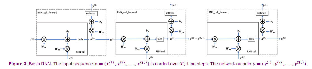
- Both ( \(W_{aa}\) ) (the weight matrix for the recurrent connection) and ( \(W_{ax}\) ) (the weight matrix for the input connection) are the same parameters used for all time steps in the sequence. This means that the same weight matrices are applied to the inputs and hidden states at each time step.
This sharing of parameters allows the RNN to efficiently learn from sequential data while reducing the number of parameters that need to be trained.
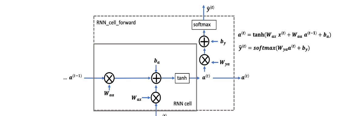
A hidden state \(a^{}\) and prediction \(y^{}\)
RNN cell versus RNN_cell_forward:
Note that an RNN cell outputs the hidden state 𝑎⟨𝑡⟩.
RNN cellis shown in the figure as the inner box with solid lines
The function that you'll implement,
rnn_cell_forward, also calculates the prediction 𝑦̂ ⟨𝑡⟩RNN_cell_forwardis shown in the figure as the outer box with dashed lines
Backpropagation Through Time
In the context of using RNNs for predictions, the loss function you choose depends on the nature of your output. If you're predicting continuous values (like temperature), you typically use a loss function like Mean Squared Error (MSE). However, if you're dealing with binary classification tasks (like predicting whether it will rain or not), you would use a logistic loss, also known as binary cross-entropy loss.
For Continuous Predictions (e.g., Weather Forecasting):
Loss Calculation: You would calculate the difference between the predicted values and the actual measured values for each time step. The loss function would be:
Mean Squared Error (MSE): \(\text{MSE} = \frac{1}{N} \sum_{i=1}^{N} (y_{\text{pred}, i} - y_{\text{true}, i})^2\)
Here, (N) is the number of predictions(or samples), \((y_{\text{pred}, i} - y_{\text{true}, i})^2\): the squared error between predicted and true values for sample
i
For Binary Classification (e.g., Rain Prediction):
Loss Calculation: If you are predicting a binary outcome (like whether it will rain), you would calculate the logistic loss for each time step:
Binary Cross-Entropy Loss: \(\begin{equation} \mathcal{L}_{\text{BCE}} = -\frac{1}{N} \sum_{i=1}^{N} \left[ y_i \log(\hat{y}_i) + (1 - y_i) \log(1 - \hat{y}_i) \right] \end{equation}\)
Here, \(\hat{y}_i\) is the predicted probability of the positive class, and \(y_i\) is the actual label (0 or 1).
Summary:
For predicting continuous values (like temperature), use MSE.
For binary outcomes (like rain/no rain), use binary cross-entropy.
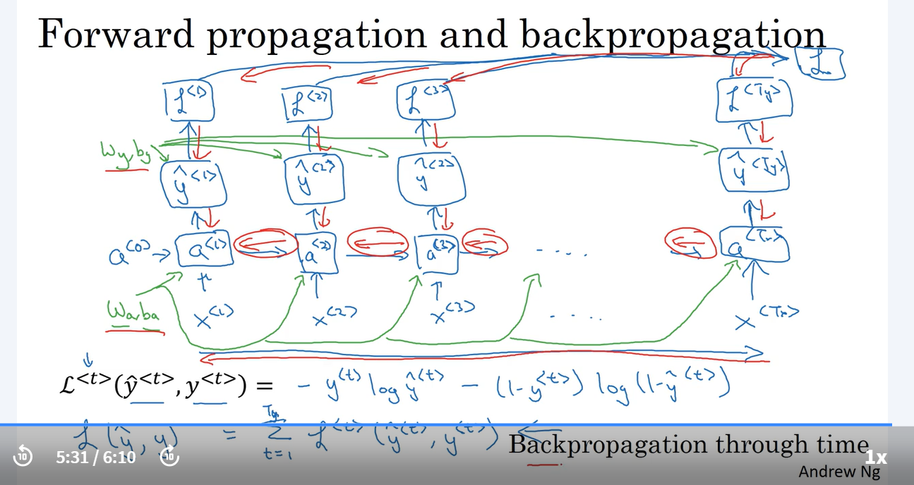
for forward propagation, you scanning from the left to right, but the backward propagation, you scanning from the right to left. you are kind of going backwards in time. so it is called back propagation through time.
Forward:
calculating the each time step loss, and sum them up, getting an overall Loss
Note:
the standard logistic regression loss, also called the cross entropy loss.
Different Types of RNNs
input and output may have different length, for instance: translating from English to French.
the presentation in this video was inspired by a blog post by Andrej Karpathy,
titled, The Unreasonable Effectiveness of Recurrent Neural Networks.
Examples of RNN architectures
Tx = Ty (many to many)
Tx to one (many to one)Sentiment classification
x = text y = 0 or 1
In a many-to-many architecture for Recurrent Neural Networks (RNNs), there are two main cases:
Input Length Equal to Output Length:
- In this case, the number of inputs (Tx) is the same as the number of outputs (Ty). An example is named entity recognition, where each input word corresponds to an output label.
Input Length Not Equal to Output Length:
- Here, the input and output sequences can have different lengths. A common example is machine translation, where a sentence in one language (e.g., French) may translate to a sentence in another language (e.g., English) that has a different number of words.
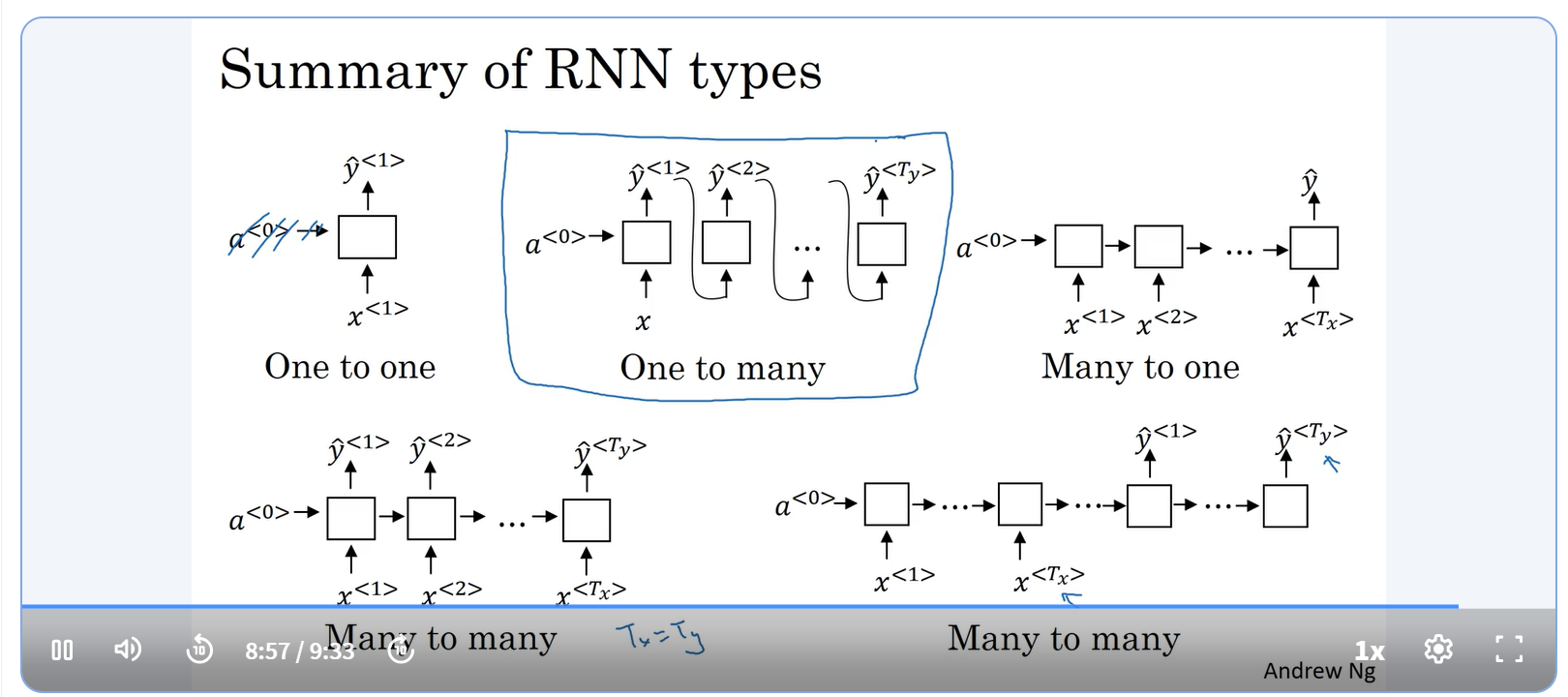
In the world of Recurrent Neural Networks (RNNs), a many-to-many architecture is like a conversation where multiple questions lead to multiple answers. Imagine you're at a party, and you ask a series of questions to your friend, and for each question, they give you a response. This is similar to how many-to-many architectures work, where you have a sequence of inputs and a sequence of outputs.
Equal Lengths:
- Think of a situation where you’re translating a poem from one language to another. Each line in the original poem corresponds to a line in the translated version. Here, the number of lines (inputs) is the same as the number of lines (outputs). This is like a game of matching pairs!
Unequal Lengths:
- Now, consider a scenario where you’re summarizing a book. You read several chapters (inputs), but your summary might only be a few sentences (output). In this case, the number of chapters you read is different from the number of sentences in your summary. This is like condensing a long story into a short one!
The many-to-many architecture differs from other architectures in the following ways:
Many-to-One Architecture:
Description: In this setup, multiple inputs lead to a single output.
Example: Sentiment analysis, where a sequence of words (input) is analyzed to produce one sentiment score (output), like positive or negative.
One-to-Many Architecture:
Description: Here, a single input generates multiple outputs.
Example: Music generation, where one note or a genre input leads to a sequence of musical notes as output.
One-to-One Architecture:
Description: This is the simplest form, where one input corresponds to one output.
Example: A standard feedforward neural network, where a single feature input results in a single prediction output.
Many-to-Many Architecture:
Description: In this architecture, multiple inputs can produce multiple outputs. This can be further divided into:
Equal Lengths: The number of inputs matches the number of outputs (e.g., named entity recognition).
Unequal Lengths: The number of inputs does not match the number of outputs (e.g., machine translation).
In summary, the key difference lies in how inputs and outputs are related in terms of quantity. Many-to-many architectures allow for flexibility in handling sequences where both input and output can vary in length, while the other architectures have more defined relationships between input and output.
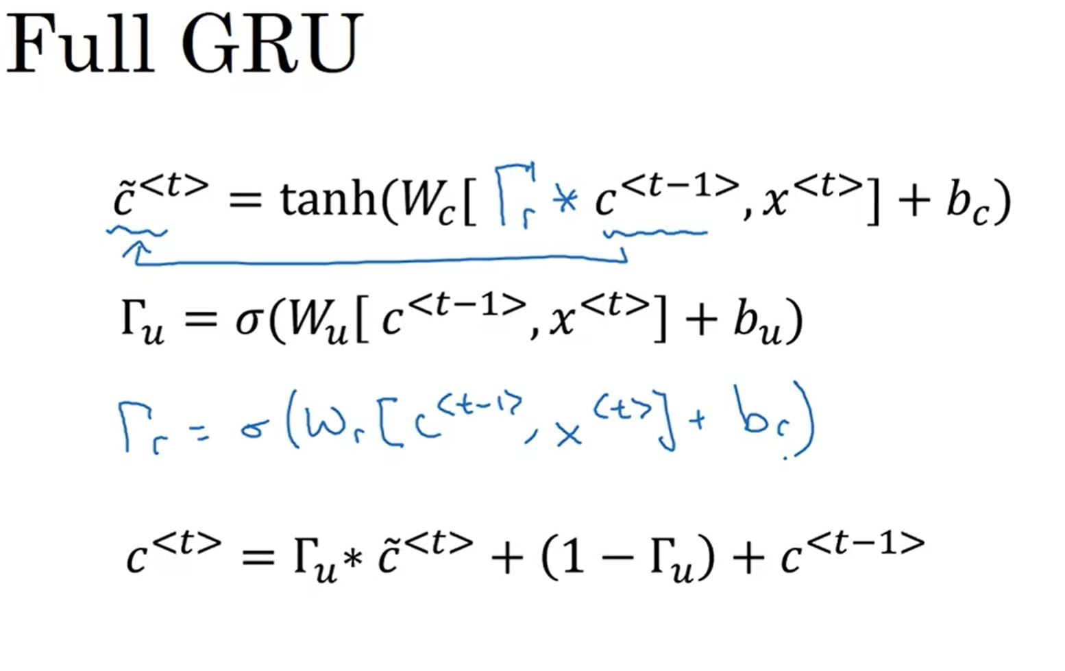
Gated Recurrent Unit (GRU)
In a Gated Recurrent Unit (GRU), the update gate (Γ_u) determines how much of the previous hidden state should be retained and how much of the new candidate hidden state should be incorporated.
Here's how it works:
Update Gate (Γ_u): This gate takes a value between 0 and 1:
A value close to 1 means that the model should mostly use the new candidate hidden state, effectively updating the hidden state.
A value close to 0 means that the model should retain the previous hidden state, minimizing the update.
The update process can be summarized as follows:
a^t = (1 - Γ_u) * a^(t-1) + Γ_u * c^t
Where:
\(a^t\) is the updated hidden state at time step t.
\(c^t\) is the candidate hidden state computed from the current input and the previous hidden state.
This mechanism allows GRUs to effectively manage long-range dependencies and adapt to new information while retaining relevant context.
Long term Short Term Memory (LSTM)
The key mental model you can keep is:
Vanilla RNN → memory is like writing on a whiteboard that keeps getting erased every step.
LSTM → adds a “long-term notebook” (cell state) that you can keep writing in, erasing only when needed.
Hidden state → still exists, but more like the scratchpad for immediate calculations.
That separation is what made LSTMs such a big breakthrough for machine translation, speech recognition, and sequential tasks before Transformers came along.
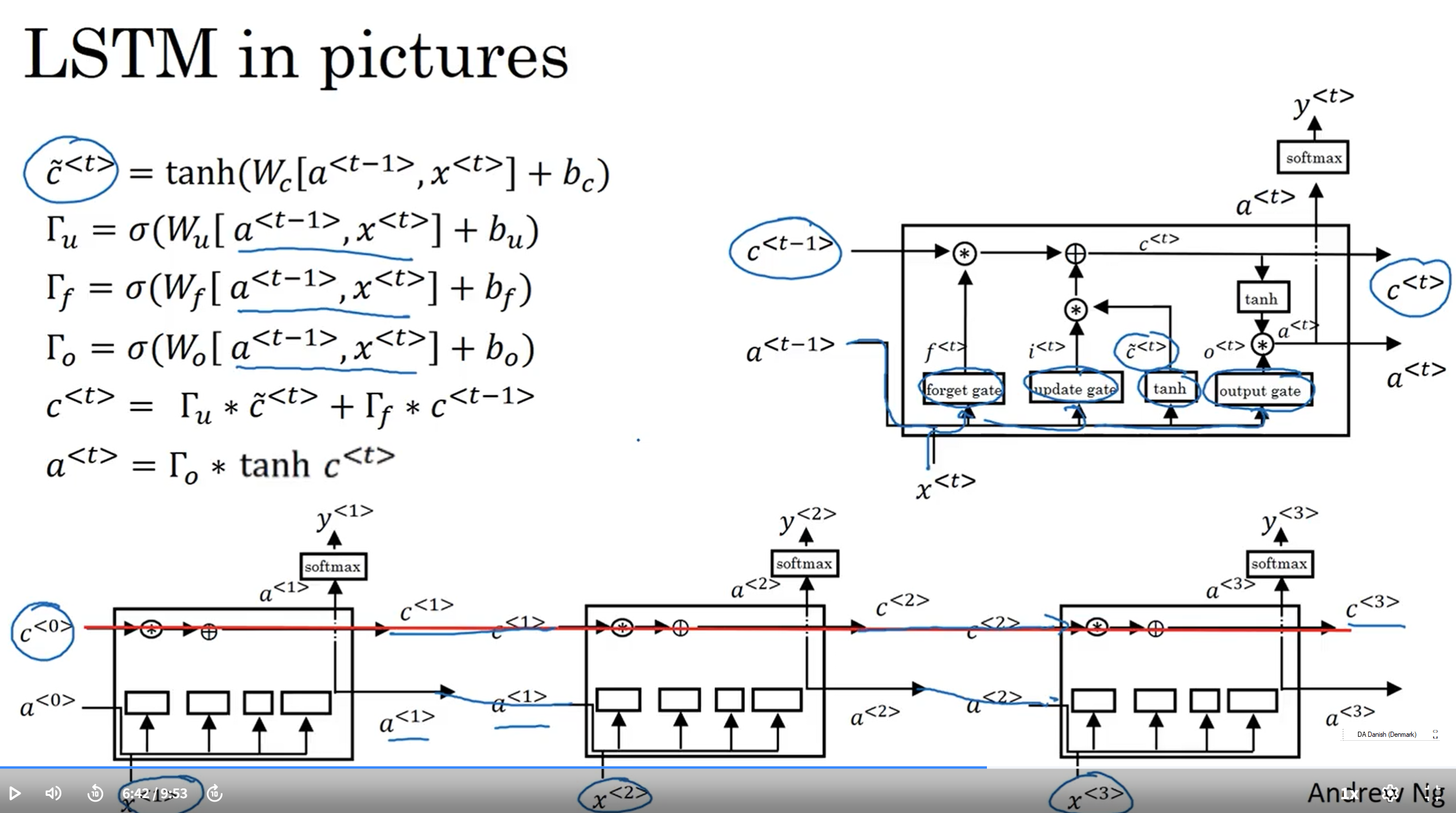
The following figure shows the operations of an LSTM cell:
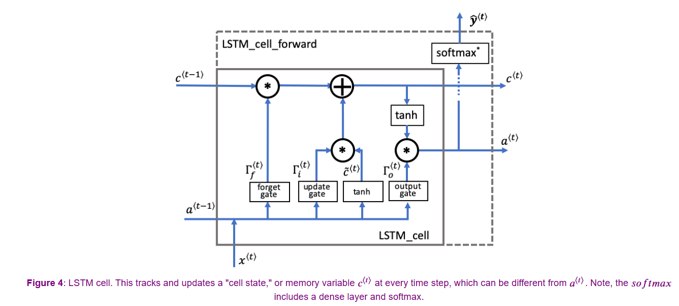
Overview of gates and states
Forget gate \(\Gamma_f \)
Let's assume you are reading words in a piece of text, and plan to use an LSTM to keep track of grammatical structures, such as whether the subject is singular ("puppy") or plural ("puppies").
If the subject changes its state (from a singular word to a plural word), the memory of the previous state becomes outdated, so you'll "forget" that outdated state.
The "forget gate" is a tensor containing values between 0 and 1.
If a unit in the forget gate has a value close to 0, the LSTM will "forget" the stored state in the corresponding unit of the previous cell state.
If a unit in the forget gate has a value close to 1, the LSTM will mostly remember the corresponding value in the stored state.
Equation (1)
$$𝚪^{⟨𝑡⟩}_𝑓=𝜎(𝐖_𝑓[𝐚^{⟨𝑡−1⟩},𝐱^{⟨𝑡⟩}]+𝐛_𝑓) (1)$$
Explanation of the equation:
\(𝐖_𝐟\) contains weights that govern the forget gate's behavior.
The previous time step's hidden state [\(𝑎^{⟨𝑡−1⟩}\) and current time step's input \(𝑥^{⟨𝑡⟩}\)] are concatenated together(vertical stack) and multiplied(np.dot) by \(𝐖_𝐟\).
A sigmoid function is used to make each of the gate tensor's values \(𝚪^{⟨𝑡⟩}_𝑓\)range from 0 to 1.
The forget gate \(𝚪^{⟨𝑡⟩}_𝑓\) has the same dimensions as the previous cell state \(𝑐^{⟨𝑡−1⟩}\).
This means that the two can be multiplied together, element-wise.
Multiplying the tensors \(𝚪^{⟨𝑡⟩}_𝑓∗𝐜^{⟨𝑡−1⟩}\) is like applying a mask over the previous cell state.
If a single value in \(𝚪^{⟨𝑡⟩}_𝑓\) is 0 or close to 0, then the product is close to 0.
- This keeps the information stored in the corresponding unit in \(𝐜^{⟨𝑡−1⟩}\) from being remembered for the next time step.
Similarly, if one value is close to 1, the product is close to the original value in the previous cell state.
- The LSTM will keep the information from the corresponding unit of \(𝐜^{⟨𝑡−1⟩}\), to be used in the next time step.
Variable names in the code
The variable names in the code are similar to the equations, with slight differences.
\(W_f\): forget gate weight
\(b_f\): forget gate bias
\(Γ_𝑓\): forget gate
Candidate value \(𝐜̃ ^{⟨𝑡⟩}\)
The candidate value is a tensor containing information from the current time step that may be stored in the current cell state \(𝐜^{⟨𝑡⟩}\).
The parts of the candidate value that get passed on depend on the update gate.
The candidate value is a tensor containing values that range from -1 to 1.
The tilde "~" is used to differentiate the candidate \(𝐜̃ ^{⟨𝑡⟩}\) from the cell state \(𝐜^{⟨𝑡⟩}\) .
Equation (3)
\[𝐜̃^{⟨𝑡⟩}=tanh(𝐖_𝑐[𝐚^{⟨𝑡−1⟩},𝐱^{⟨𝑡⟩}]+𝐛_𝑐)(3)\]
Explanation of the equation
- The tanh function produces values between -1 and 1.
Variable names in the code
cct: candidate value \(𝐜̃ ^{⟨𝑡⟩}\)
Update gate \(𝚪_𝑖\)
You use the update gate to decide what aspects of the candidate \(𝐜̃^{⟨𝑡⟩}\) to add to the cell state 𝑐⟨𝑡⟩.
The update gate decides what parts of a "candidate" tensor \(𝐜̃ ^{⟨𝑡⟩}\) are passed onto the cell state \( 𝑐^{⟨𝑡⟩}\) .
The update gate is a tensor containing values between 0 and 1.
When a unit in the update gate is close to 1, it allows the value of the candidate 𝐜̃ ⟨𝑡⟩ to be passed onto the hidden state 𝐜⟨𝑡⟩
When a unit in the update gate is close to 0, it prevents the corresponding value in the candidate from being passed onto the hidden state.
Notice that the subscript "i" is used and not "u", to follow the convention used in the literature.
Equation (2)
𝚪𝑖⟨𝑡⟩=𝜎(𝐖𝑖[𝑎⟨𝑡−1⟩,𝐱⟨𝑡⟩]+𝐛𝑖)(2)
Explanation of the equation
Similar to the forget gate, here 𝚪⟨𝑡⟩𝑖, the sigmoid produces values between 0 and 1.
The update gate is multiplied element-wise with the candidate, and this product (𝚪⟨𝑡⟩𝑖∗𝑐̃ ⟨𝑡⟩) is used in determining the cell state 𝐜⟨𝑡⟩.
Variable names in code (Please note that they're different than the equations)
In the code, you'll use the variable names found in the academic literature. These variables don't use "u" to denote "update".
Wiis the update gate weight 𝐖𝑖biis the update gate bias 𝐛𝑖itis the update gate 𝚪⟨𝑡⟩𝑖
Cell state 𝐜⟨𝑡⟩
The cell state is the "memory" that gets passed onto future time steps.
The new cell state 𝐜⟨𝑡⟩ is a combination of the previous cell state and the candidate value.
Equation
𝐜⟨𝑡⟩=𝚪⟨𝑡⟩𝑓∗𝐜⟨𝑡−1⟩+𝚪⟨𝑡⟩𝑖∗𝐜̃ ⟨𝑡⟩(4)
Explanation of equation
The previous cell state 𝐜⟨𝑡−1⟩ is adjusted (weighted) by the forget gate 𝚪⟨𝑡⟩𝑓
and the candidate value 𝐜̃ ⟨𝑡⟩, adjusted (weighted) by the update gate 𝚪⟨𝑡⟩𝑖
Variable names and shapes in the code
c: cell state, including all time steps, 𝐜 shape (𝑛𝑎,𝑚,𝑇𝑥)c_next: new (next) cell state, 𝐜⟨𝑡⟩ shape (𝑛𝑎,𝑚)c_prev: previous cell state, 𝐜⟨𝑡−1⟩, shape (𝑛𝑎,𝑚)
Output gate 𝚪𝑜
The output gate decides what gets sent as the prediction (output) of the time step.
The output gate is like the other gates, in that it contains values that range from 0 to 1.
Equation
𝚪⟨𝑡⟩𝑜=𝜎(𝐖𝑜[𝐚⟨𝑡−1⟩,𝐱⟨𝑡⟩]+𝐛𝑜)(5)
Explanation of the equation
The output gate is determined by the previous hidden state 𝐚⟨𝑡−1⟩ and the current input 𝐱⟨𝑡⟩
The sigmoid makes the gate range from 0 to 1.
Variable names in the code
Wo: output gate weight, 𝐖𝐨bo: output gate bias, 𝐛𝐨ot: output gate, 𝚪⟨𝑡⟩𝑜
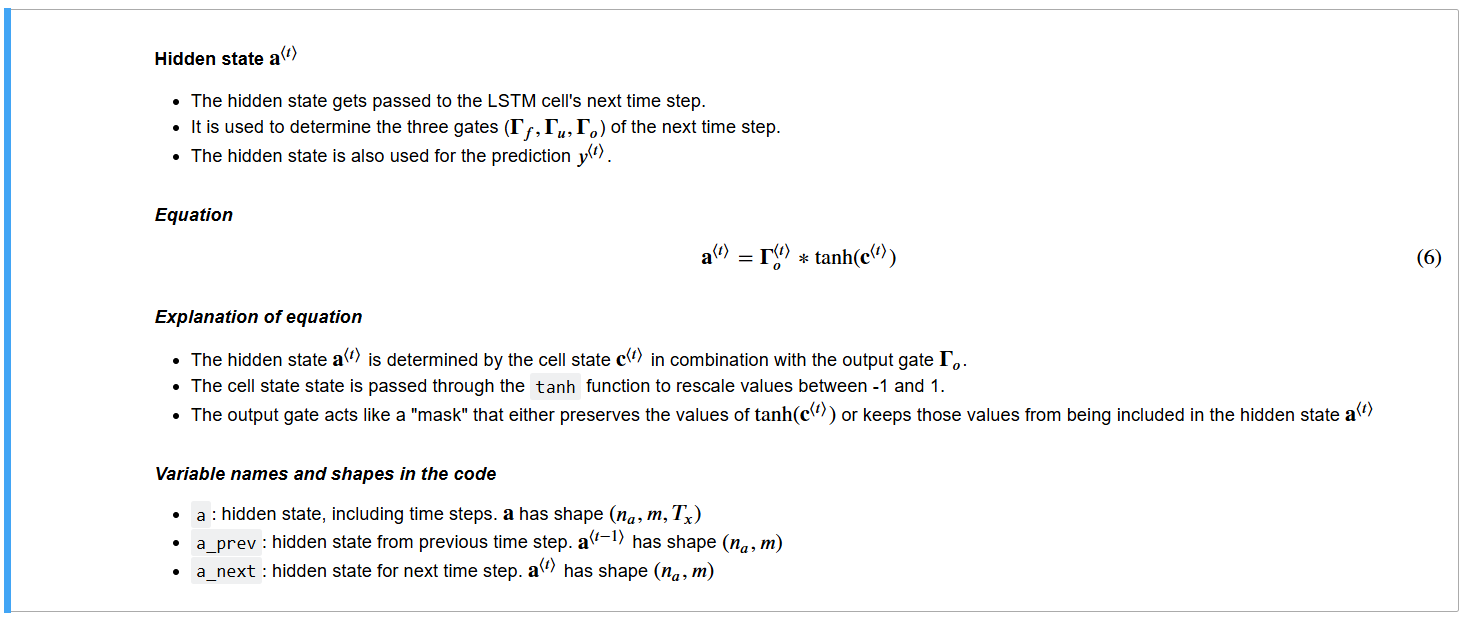
Hidden state 𝐚⟨𝑡⟩ -next hidden state
The hidden state gets passed to the LSTM cell's next time step.
It is used to determine the three gates (𝚪𝑓,𝚪𝑢,𝚪𝑜) of the next time step.
The hidden state is also used for the prediction 𝑦⟨𝑡⟩.
Equation
$$𝐚⟨𝑡⟩=𝚪^{⟨𝑡⟩}_𝑜∗tanh(𝐜^{⟨𝑡⟩}) (6)$$
Explanation of equation
The hidden state ( 𝐚^{⟨𝑡⟩} ) is determined by the cell state 𝐜⟨𝑡⟩ in combination with the output gate 𝚪𝑜.
The cell state state is passed through the
tanhfunction to rescale values between -1 and 1.The output gate acts like a "mask" that either preserves the values of tanh(𝐜⟨𝑡⟩) or keeps those values from being included in the hidden state 𝐚⟨𝑡⟩
Variable names and shapes in the code
a: hidden state, including time steps. 𝐚 has shape (𝑛𝑎,𝑚,𝑇𝑥)a_prev: hidden state from previous time step. 𝐚⟨𝑡−1⟩ has shape (𝑛𝑎,𝑚)a_next: hidden state for next time step. 𝐚⟨𝑡⟩ has shape (𝑛𝑎,𝑚)
Prediction \(𝐲^{⟨𝑡⟩}_{𝑝𝑟𝑒𝑑}\)
- The prediction in this use case is a classification, so you'll use a softmax.
The equation is:
$$𝐲^{⟨𝑡⟩}{𝑝𝑟𝑒𝑑}=softmax(𝐖{𝑦𝐚}^{⟨𝑡⟩}+𝐛_𝑦)$$
Variable names and shapes in the code
y_pred: prediction, including all time steps. 𝐲𝑝𝑟𝑒𝑑 has shape (𝑛𝑦,𝑚,𝑇𝑥). Note that (𝑇𝑦=𝑇𝑥) for this example.yt_pred: prediction for the current time step 𝑡. 𝐲⟨𝑡⟩𝑝𝑟𝑒𝑑 has shape (𝑛𝑦,𝑚)
2.1 - LSTM Cell
Exercise 3 - lstm_cell_forward
Implement the LSTM cell described in Figure 4.
Instructions:
- Concatenate the hidden state 𝑎⟨𝑡−1⟩ and input 𝑥⟨𝑡⟩ into a single matrix:
𝑐𝑜𝑛𝑐𝑎𝑡=[𝑎⟨𝑡−1⟩𝑥⟨𝑡⟩]
Compute all formulas (1 through 6) for the gates, hidden state, and cell state.
Compute the prediction 𝑦⟨𝑡⟩.
Additional Hints
You can use numpy.concatenate. Check which value to use for the
axisparameter.The functions
sigmoid()andsoftmaxare imported fromrnn_utils.py.Some docs for numpy.tanh
Use numpy.dot for matrix multiplication.
Notice that the variable names
Wi,birefer to the weights and biases of the update gate. There are no variables named "Wu" or "bu" in this function.
An LSTM (Long Short-Term Memory) cell contains two states:
🧠 1. Hidden State (h_t)
This is the "output" of the LSTM at time step t.
It gets passed to the next time step and can also be used for predictions.
🧠 2. Cell State (or Memory State) (c_t)
This is the long-term memory of the LSTM.
It flows through the sequence with minor linear interactions (modified slightly at each time step), making it easier to preserve information over long ranges.
Why two states?
The motivation is to overcome the vanishing gradient problem in standard RNNs. The cell state ctc_t acts like a "conveyor belt" that allows gradients and information to flow more easily across many time steps.
Summary of LSTM Workflow (at each time step t):
Input: current input x_t, previous hidden state h_{t-1}, and previous cell state c_{t-1}
Gates:
Forget gate: decides what part of c_{t-1} to forget
Input gate: decides what new information to add
Output gate: controls what to output as h_t
Cell update: combine old and new info → get c_t
Hidden state update: based on c_t, get h_t
Diagram (simplified view):
          c_{t-1} ------------------> [Forget] -----
               |                            |      |
               v                            ↓      v
x_t, h_{t-1} ->[Input]--> [New Info] --> [+] --> c_t --> [Output Gate] --> h_t
Great question — you're asking the right kind of "deep" question here.
🧠 So: What does a value between -1 and 1 in the hidden state actually mean or how is it interpreted?
📦 The hidden state is a vector of features — not probabilities.
Each element in the hidden state vector (say, ht∈Rnh_t \in \mathbb{R}^n) represents a learned feature or signal the network uses to store and transmit information across time.
A value near 0:
→ That feature is inactive or not significant at this time step.A value close to +1 or -1:
→ That feature is strongly active, either positively (+) or negatively (–).
⚖️ Why both negative and positive?
Using an activation like tanh (which outputs in [−1,1][-1, 1]) instead of sigmoid ([0,1][0, 1]) is intentional:
It allows the network to express positive or negative correlations, or excitation vs inhibition.
A negative value can "cancel out" or suppress something when passed forward.
This gives richer representation capacity than just values between 0 and 1.
🔁 Example:
Imagine you're doing sentiment analysis over a sentence like:
"I don't think this movie was good."
The hidden state at each time step might encode:
| Feature index | Meaning (learne | h_t value |
| 0 | "Is the tone negative?" | +0.9 |
| 1 | "Is there sarcasm?" | -0.7 |
| 2 | "Was there strong emotion?" | +0.3 |
These aren't human-interpretable directly — but over training, the model learns to use combinations of these values to make decisions.
📉 In downstream tasks:
The final hidden state (or all of them) may be passed into:
A fully connected (dense) layer
Possibly followed by SoftMax or Sigmoid
Which gives you interpretable probabilities, class labels, etc.
So:
Hidden state values themselves aren't probabilities. They are learned, real-valued features used internally to model temporal dependencies.
✅ TL;DR:
Hidden state values in [-1, 1] are feature activations, not probabilities.
Negative values are meaningful — they help the network express rich patterns.
Interpretation comes indirectly by how the network uses them, not by direct human labels.
Let me know if you want a visualization or step-by-step example with code!
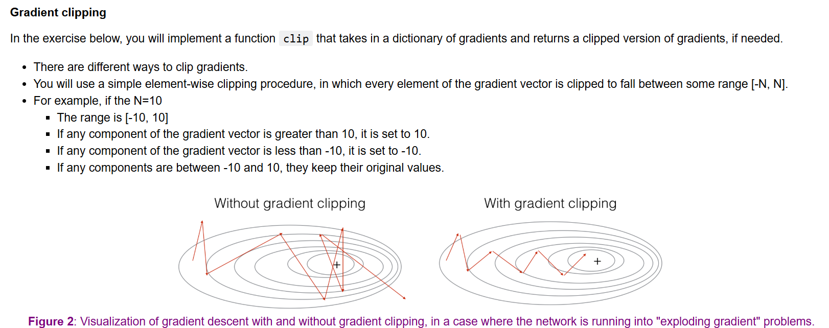
Gradient Exploding
solution to gradient explosion, it is simple and direct compared with the momentum method.
### START CODE HERE ###
    # Clip to mitigate exploding gradients, loop over [dWax, dWaa, dWya, db, dby]. (≈2 lines)
    for gradient in [dWaa, dWax, dWya, db, dby]:
        np.clip(gradient, -maxValue, maxValue, out = gradient)
    ### END CODE HERE ###
Building LM
building a character-level LM for text generation.
Gradient Descent
stochastic gradient decent(SGD) with gradient clip. Go through the training examples one at a time.
Forward propagation through RNN to compute Loss(cross-entropy loss, cache values)
Backward propagation through time to compute the grad. of the loss with respect to the parameter(grad. with respect to the parameters, hidden states).
Clip the gradients
Updating RNN model parameters using gradient descent
vocab_size = by.shape[0] : the number of vocabulary.
n_a = Waa.shape[1 ] : number of units of the RNN cell, which is used to describe the hidden state.
n_x : number of features in input \( X^{}\), which eq. to vocab_size.
n_e: number of examples
Implement model()
When examples[index] contains one dinosaur name (string), to create an example (X, Y), you can use this:
using for-loop to traverse the shuffled list of dinosaur names(examples) using index.
Converting a string into a list of characters: single_example_chars, i.e. a list of characters.
Converting list of characters to a list of integers(idx): single_example_ix using char_to_ix.
Creating the list of input characters: x, none stands for a zero-vector,
prepend the list[None] in the form of the list of input character indices, [‘a‘]+[‘b‘]
ix_newline Use char_to_ix
Label list Y (integer representation of the character)
"What the RNN model learns from the training set is the sequential dependency pattern. Although X and Y contain almost the same characters, the RNN captures how characters depend on each other over time."
Goal: Train a Recurrent Neural Network (RNN) to predict the next letter in a name.
Input (X): A list of integer representations of characters (letters) in the name.
Labels (Y): A list of integer representations of characters that are one time-step ahead of the characters in X.
How to create Y:
- Take the integer representation of each character in X and shift it one position forward to create Y. This means Y[0] will have the same value as X[1], Y[1] will have the same value as X[2], and so on.
Special case: When the RNN reaches the last letter, it should predict a newline character. To achieve this:
- Append the integer representation of the newline character (ix_newline) to the end of Y.
Important note: The append operation modifies the list in-place, meaning it changes the original list without creating a new one.
Example:
If X = [1, 2, 3, 4] (representing the letters "ABCD"), then Y would be [2, 3, 4, ix_newline] (representing the letters "BCD\n").
Improvise a Jazz Solo with an LSTM Network
Apply an LSTM to a music generation task
Generate your own jazz music with deep learning
Use the flexible Functional API to create complex models
Problem Statement
Given a corpus of Jazz music, and use them to train a LTSM model 😎🎷. Then use it to generate Jazz, by giving the model a initial which is not usually a zero vector in generation — instead, it's often:
A seed note (e.g., MIDI pitch 60)
Or an embedding of a seed character or value
chord: when press down two piano keys at the same time (playing multiple notes at the same time generates what's called a "chord".
value: informally seen as a note, which consists of a pitch and its duration. For example, if you press down a specific piano key for 0.5 seconds, then you have played a note.
Keras(a part of Tensorflow) is an open-source, high-level deep learning API (Application Programming Interface). Its main purpose is to make building and training neural networks simple and fast, especially for beginners and researchers who want to prototype ideas quickly. It provides layers, models, optimizers and utils.
# number of dimensions for the hidden state of each LSTM cell.
n_a = 64
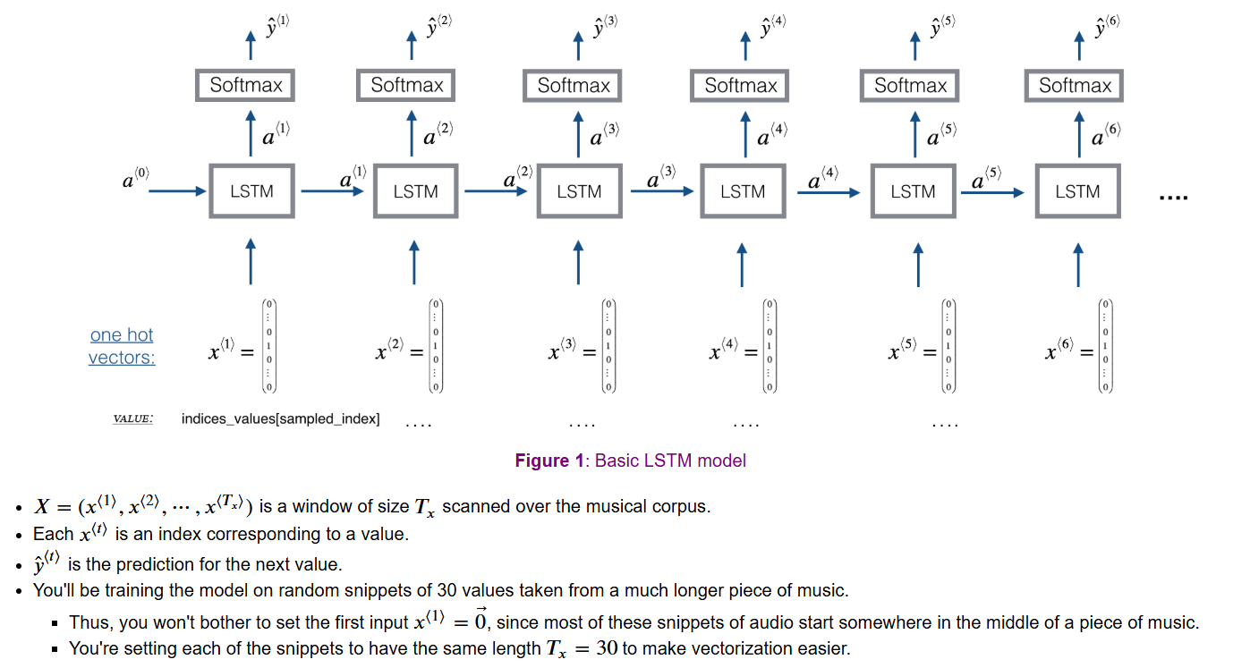
n_x = 90; Tx = 30; m=60; Tx = Ty;
- The model takes input X of shape (𝑚,𝑇𝑥,90) and labels Y of shape (𝑇𝑦,𝑚,90).
Implement djmodel()
in the context of djmodel() for music generation, Keras provides abstractions for the input, LSTM, and Dense layers, which are the core components used to build the model.
Each cell has the following schema: \([X_{t}, a_{t-1}, c0_{t-1}] \rightarrow RESHAPE() \rightarrow LSTM() \rightarrow DENSE()\)
LSTM : implementation of a Cell
DENSE: implementation of soft-max output
# UNQ_C1 (UNIQUE CELL IDENTIFIER, DO NOT EDIT)
# GRADED FUNCTION: djmodel

def djmodel(Tx, LSTM_cell, densor, reshaper):
    """
    Implement the djmodel composed of Tx LSTM cells where each cell is responsible
    for learning the following note based on the previous note and context.
    Each cell has the following schema:
            [X_{t}, a_{t-1}, c0_{t-1}] -> RESHAPE() -> LSTM() -> DENSE()
    Arguments:
        Tx -- length of the sequences in the corpus
        LSTM_cell -- LSTM layer instance
        densor -- Dense layer instance
        reshaper -- Reshape layer instance

    Returns:
        model -- a keras instance model with inputs [X, a0, c0]
    """
    # Get the shape of input values
    n_values = densor.units

    # Get the number of the hidden state vector
    n_a = LSTM_cell.units

    # Define the input layer and specify the shape
    X = Input(shape=(Tx, n_values))

    # Define the initial hidden state a0 and initial cell state c0
    # using `Input`
    a0 = Input(shape=(n_a,), name='a0')
    c0 = Input(shape=(n_a,), name='c0')
    a = a0
    c = c0
    ### START CODE HERE ###
    # Step 1: Create empty list to append the outputs while you iterate (≈1 line)
    outputs = []

    # Step 2: Loop over tx
    for t in range(Tx):

        # Step 2.A: select the "t"th time step vector from X.
        x = X[:,t,:]
        # Step 2.B: Use reshaper to reshape x to be (1, n_values) (≈1 line)
        x = reshaper(x)
        # Step 2.C: Perform one step of the LSTM_cell
        _, a, c = LSTM_cell(inputs=x, initial_state=[a, c])
        # Step 2.D: Apply densor to the hidden state output of LSTM_Cell
        out = densor(a)
        # Step 2.E: append the output to "outputs"
        outputs.append(out)

    # Step 3: Create model instance
    model = Model(inputs=[X, a0, c0], outputs=outputs)

    ### END CODE HERE ###

    return model
Compile the model for training
You now need to compile your model to be trained.
We will use:
Optimizer: Adam optimizer
Loss function: categorical cross-entropy (for multi-class classification).
‘categorical_crossentropy’: This is used when your output is a probability distribution over multiple classes (e.g., SoftMax output) and your labels are one-hot encoded.
opt = Adam(lr=0.01, beta_1=0.9, beta_2=0.999, decay=0.01)

model.compile(optimizer=opt, loss='categorical_crossentropy', metrics=['accuracy'])
Initialize hidden state and cell state
Finally, let's initialize a0 and c0 for the LSTM's initial state to be zero.
    m = 60
# when trainning the model, we use 0 vectors
a0 = np.zeros((m, n_a))
c0 = np.zeros((m, n_a))
# training model
history = model.fit([X, a0, c0], list(Y), epochs=100, verbose = 0)
Generating Music
Predicting and Sampling
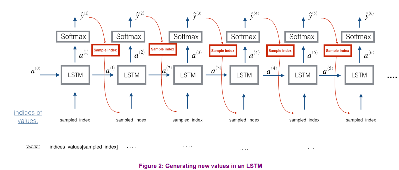
when using trained LSTM to generate Jazz, the sampling process happens in this process. that is why each time when using initial value to generate the music, the result maybe different.
At each step of sampling, you will:
Take as input the activation '
a' and cell state 'c' from the previous state of the LSTM.Forward propagate by one step.
Get a new output activation, as well as cell state.
The new activation '
a' can then be used to generate the output using the fully connected layer,densor.
Initialization
You'll initialize the following to be zeros:
x0hidden state
a0cell state
c0
# UNQ_C2 (UNIQUE CELL IDENTIFIER, DO NOT EDIT)
# GRADED FUNCTION: music_inference_model

def music_inference_model(LSTM_cell, densor, Ty=100):
    """
    Uses the trained "LSTM_cell" and "densor" from model() to generate a sequence of values.

    Arguments:
    LSTM_cell -- the trained "LSTM_cell" from model(), Keras layer object
    densor -- the trained "densor" from model(), Keras layer object
    Ty -- integer, number of time steps to generate

    Returns:
    inference_model -- Keras model instance
    """

    # Get the shape of input values
    n_values = densor.units
    # Get the number of the hidden state vector
    n_a = LSTM_cell.units

    # Define the input of your model with a shape
    x0 = Input(shape=(1, n_values))


    # Define s0, initial hidden state for the decoder LSTM
    a0 = Input(shape=(n_a,), name='a0')
    c0 = Input(shape=(n_a,), name='c0')
    a = a0
    c = c0
    x = x0

    ### START CODE HERE ###
    # Step 1: Create an empty list of "outputs" to later store your predicted values (≈1 line)
    outputs = []

    # Step 2: Loop over Ty and generate a value at every time step
    for t in range(Ty):
        # Step 2.A: Perform one step of LSTM_cell. Use "x", not "x0" (≈1 line)
        _, a, c = LSTM_cell(x, initial_state=[a, c])

        # Step 2.B: Apply Dense layer to the hidden state output of the LSTM_cell (≈1 line)
        out = densor(a)
        # Step 2.C: Append the prediction "out" to "outputs". out.shape = (None, 90) (≈1 line)
        outputs.append(out)

        # Step 2.D:
        # Select the next value according to "out",
        # Set "x" to be the one-hot representation of the selected value
        # See instructions above.
        x = tf.math.argmax(out,axis=1)
        x = tf.onehot(x, depth=n_values)
        # Step 2.E:
        # Use RepeatVector(1) to convert x into a tensor with shape=(None, 1, 90)
        x = RepeatVector(1)(x)

    # Step 3: Create model instance with the correct "inputs" and "outputs" (≈1 line)
    inference_model = None

    ### END CODE HERE ###

    return inference_model